Introduction

ViT is a transformer model for computer vision. In this post, I write some code to apply the model to MNIST and compare its performance against a CNN. The basic idea behind a visual transformer is to chop the images into sections and pass each section, along with a trainable position embedding and trainable class embedding to the transformer.

Variables

Lets define some parameters before defining the model.

Paramater	Value
Image Height	\(H\)
Image Width	\(W\)
Image Channels	\(C\)
Image Patch Size	\(P\)
Image	\(x \in \mathcal{R}^{H \times W \times C}\)
Image Patch	\(x_p \in \mathcal{R}^{N \times (P^2C)}\)
Number of Patches	\(N=\frac{HW}{P^2}\)
Transformer Latent Vector Size	\(D\)
Number of Layers	\(L\)

Model

Lets define some parameters for the model.

Parameter	Variable
Transformer Latent Vector Size	\(D\)
Number of Attention Layers	\(L\)
Learnable Class Embedding	\(x_{class}^D\)
Learnable Position Embedding	\(\boldsymbol{E}_{pos}\in\mathcal{R}^{(N + 1) \times D}\)
Linear Projector	\(\boldsymbol{E}\in\mathcal{R}^{(P^2C) \times D}\)

The original paper defines the model and its inputs like below. It’s surprisingly simple.

\[\begin{align*} & z_0 = [x_{class}^D;x_p^1\boldsymbol{E};x_p^2\boldsymbol{E};\dots;x_p^N\boldsymbol{E}] + \boldsymbol{E}_{pos}\\ & z_l^{'} = MultiHeadSelfAttention(LayerNorm(z_{l-1})) + z_{l-1}\qquad l=1...L\\ & z_l = MultiLayerPerceptron(LayerNorm(z_{l-1}^{'})) + z_l^{'} \qquad l=1...L\\ & y = LayerNorm(z_{L}^0) \end{align*}\]

We construct \(z_0\), with the class embedding, the linear projection on the image patches and the position embedding. Next, we pass this data to the transformer layers. At the end, we examine the first token to determine the class of the image.

Data Preperation

MNIST

Lets prepare the data according to the following parameters.

Parameter	Value
H	28
W	28
C	1
P	7
N	16

Based on these parameters, we can construct image patches with the following dimensions.

\[x = \mathcal{R}^{28 \times 28} \rightarrow x_p = \mathcal{R}^{16 \times 49}\]

If we define a patch size of \(P = 7 x 7\), then we will have 16 patches which are flattened to construct inputs of dimension 16 x 49.

Code

Data

Lets load the MNIST data for the CNN and the ViT model. The data for the CNN is straight forward using pytorch. For the ViT model, we introduce a function to chop the images into image patches.

CNN

def load_data_cnn():
    trainset = torchvision.datasets.MNIST(DATA_DIR, True, download=True, transform=torchvision.transforms.Compose([
        torchvision.transforms.ToTensor(),
        torchvision.transforms.Normalize(
            (0.1307,), (0.3081,))
    ]))
    trainloader = torch.utils.data.DataLoader(
        trainset, batch_size=BATCH_SIZE, shuffle=True)
    testset = torchvision.datasets.MNIST(DATA_DIR, False, download=True, transform=torchvision.transforms.Compose([
        torchvision.transforms.ToTensor(),
        torchvision.transforms.Normalize(
            (0.1307,), (0.3081,))
    ]))
    testloader = torch.utils.data.DataLoader(
        testset, batch_size=BATCH_SIZE, shuffle=True
    )
    return trainloader, testloader

ViT

def load_data_ViT():
    trainset = torchvision.datasets.MNIST(DATA_DIR, True, download=True, transform=torchvision.transforms.Compose([
        torchvision.transforms.ToTensor(),
        torchvision.transforms.Normalize((0.1307,), (0.3081,)),
        cut_image
    ]))
    trainloader = torch.utils.data.DataLoader(
        trainset, batch_size=BATCH_SIZE, shuffle=True)
    testset = torchvision.datasets.MNIST(DATA_DIR, False, download=True, transform=torchvision.transforms.Compose([
        torchvision.transforms.ToTensor(),
        torchvision.transforms.Normalize((0.1307,), (0.3081,)),
        cut_image
    ]))
    testloader = torch.utils.data.DataLoader(
        testset, batch_size=BATCH_SIZE, shuffle=True
    )
    return trainloader, testloader


def cut_image(image): # <--- Function for creating patches.
    image = image.squeeze()
    cuts = [torch.hsplit(img, 4) for img in torch.vsplit(image, 4)]
    DD = []
    for LL in cuts:
        for i in LL:
            DD.append(i.unsqueeze(0))
    DD = np.concatenate(DD)
    return DD

Models

CNN

I defined the CNN model for this experiment like below.

class CNN(torch.nn.Module):
    def __init__(self):
        super(CNN, self).__init__()
        self.conv1 = nn.Conv2d(1, 32, 3, 1)
        self.conv2 = nn.Conv2d(32, 64, 3, 1)
        self.dropout1 = nn.Dropout(0.25)
        self.dropout2 = nn.Dropout(0.5)
        self.fc1 = nn.Linear(9216, 128)
        self.fc2 = nn.Linear(128, 10)

    def forward(self, x):
        x = self.conv1(x)
        x = F.relu(x)
        x = self.conv2(x)
        x = F.relu(x)
        x = F.max_pool2d(x, 2)
        x = self.dropout1(x)
        x = torch.flatten(x, 1)
        x = self.fc1(x)
        x = F.relu(x)
        x = self.dropout2(x)
        x = self.fc2(x)
        output = F.log_softmax(x, dim=1)
        return output

ViT

The code for the ViT model is given below.

class ViT(torch.nn.Module):
    def __init__(self, P, N, D, H, MLP) -> None:
        super(ViT, self).__init__()
        self.D = D
        self.N = N
        self.class_random = torch.normal(0, 1, size=(1, 1, D))
        self.location_encoding = torch.tensor(
            [[i for i in range(0, 17)]], dtype=torch.int32)
        self.position_embeddings = nn.Embedding(N + 1, D)
        self.flatten = nn.Flatten(2)
        self.patch_projection = nn.Linear(P*P, D)
        self.encoder1 = nn.TransformerEncoder(
            nn.TransformerEncoderLayer(D, H, 3000, activation="gelu"),
            num_layers=4
        )
        self.mlp1 = nn.Linear(self.D, 250)
        self.mlp2 = nn.Linear(250, 100)
        self.mlp3 = nn.Linear(100, 10)
        self.amax = torch.argmax

    def forward(self, x):
        class_random = self.class_random.repeat(x.shape[0], 1, 1)
        x_loc = self.position_embeddings(self.location_encoding)
        x = self.flatten(x)
        x_p = self.patch_projection(x)
        encoding = torch.cat([class_random, x_p], dim=1) + x_loc
        encoding = F.normalize(encoding)
        z = self.encoder1(encoding) # <--- Transformer output
        head_code = z[:, 0]
        x = self.mlp1(head_code)
        x = self.mlp2(x)
        x = F.tanh(x)
        x = self.mlp3(x)
        output = F.log_softmax(x, dim=1)
        return output

Notice that we define embeddings for the position self.position_embeddings and the class self.class_random. The class embedding is initially a random vector because the class of the image is unknown when passed to the model. After the encoder, we extract the first token in the output of the transformer and pass it to a simple neural network for classification.

Training & Results

I’ve skipped over the code used for training because it’s trivial. I utilized a batch size of 32, the negative log likelihood as loss and applied stochastic gradient descent. The loss for the training and the accuracy of the models on the test dataset can be seen below.

yay

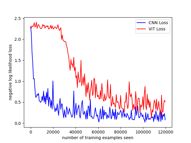
Model	Loss (NLL)	Accuracy on Test Set
CNN	0.0810	9755/10000 (98%)
ViT	0.3118	9038/10000 (90%)

Notice that the loss for the CNN is lower than the ViT. This is also reflected in the accuracy of the model on the training dataset. This CNN is still better able to extract the necessary information to classify the MNIST dataset. However, the ViT model is quite close indicating that further training epochs and parameter turning could lead to better results. I suspect that the reason the ViT has difficulty compared to the CNN is due to the fact that some information about pixel position is lost when we chop images into patches. Nonetheless, the performance of the transformer is impressive.

Ref

An Image is Worth 16X16 Words: Transformers for Image Recognition at Scale